
前回、TimesFMを使って株価を予測しました。


うまく予想できてそうな場合もありましたが、結論としては「偶然当たっただけ」ということになりました。
株価には、会社の経営状況や、商品の売れ行き、もしくは他の会社との競争などの要因があります。そのため、株価の未来予測は、根本的に無理があります。
しかし、為替はどうでしょうか?為替は株価ほど大きく変動せず、かつ安定的に保とうとする作用があります。特に日本円なんて、今は円安の状況ですが、二倍の価格変動もしていません。
もしかしたら、短期の為替予測はTimesFMでうまくいくかもしれません。
今回の記事はそれを試していく話となります。
実験 為替USDJPY 日足 短期予測
始めに日足を予測してみたいと思います。
以下jupyter notebookの記録です
まず、timesfmやyfinanceをインポートします。
import timesfm
import yfinance as yf
Appleの株価をダウンロードします。
df = yf.download(tickers='USDJPY=X', interval='1d')
df = df.reset_index().rename(columns={'Date':'ds'})
df['unique_id'] = 'USDJPY'
df
yfinanceが問題なければ、数秒でapple株の株価の記録が取得できます。
1980年からの株価が取れました。
[*********************100%%**********************]  1 of 1 completed
ds	Open	High	Low	Close	Adj Close	Volume	unique_id
0	1996-10-30	114.370003	114.480003	113.610001	114.180000	114.180000	0	USDJPY
1	1996-11-01	113.500000	113.500000	113.500000	113.500000	113.500000	0	USDJPY
2	1996-11-04	113.279999	113.980003	112.949997	113.879997	113.879997	0	USDJPY
3	1996-11-05	113.709999	114.330002	113.449997	114.250000	114.250000	0	USDJPY
4	1996-11-06	114.230003	114.680000	113.650002	113.949997	113.949997	0	USDJPY
...	...	...	...	...	...	...	...	...
7151	2024-05-28	156.845001	156.988998	156.612000	156.845001	156.845001	0	USDJPY
7152	2024-05-29	157.261993	157.639008	157.022003	157.261993	157.261993	0	USDJPY
7153	2024-05-30	157.608002	157.626999	156.427002	157.608002	157.608002	0	USDJPY
7154	2024-05-31	156.953003	157.362000	156.570007	156.953003	156.953003	0	USDJPY
7155	2024-06-02	157.289993	157.289993	157.289993	157.289993	157.289993	0	USDJPY
7156 rows × 8 columns
データが多すぎると感じたため、2015年以前は切り捨てます。また、モデルにいれるのは2024年までのデータとし、それ以降の推移を予測値と実際の値を比較します。
import pandas as pd
df['ds'] = pd.to_datetime(df['ds'])
input_df = df.loc[('2015-01-01' <= df['ds']) & (df['ds'] <= '2023-01-01'), :]
input_df
ds Open High Low Close Adj Close Volume unique_id
4701 2015-01-01 119.672997 119.672997 119.672997 119.672997 119.672997 0 USDJPY
4702 2015-01-02 119.889999 120.736000 119.835999 119.870003 119.870003 0 USDJPY
4703 2015-01-05 120.389000 120.608002 119.411003 120.433998 120.433998 0 USDJPY
4704 2015-01-06 119.416000 119.497002 118.680000 119.425003 119.425003 0 USDJPY
4705 2015-01-07 118.674004 119.639000 118.674004 118.672997 118.672997 0 USDJPY
... ... ... ... ... ... ... ... ...
7041 2023-12-26 142.229996 142.619995 142.108002 142.229996 142.229996 0 USDJPY
7042 2023-12-27 142.460999 142.832001 141.858002 142.460999 142.460999 0 USDJPY
7043 2023-12-28 141.399002 141.651993 140.289993 141.399002 141.399002 0 USDJPY
7044 2023-12-29 141.429993 141.899002 140.828995 141.429993 141.429993 0 USDJPY
7045 2024-01-01 140.951996 141.024994 140.951996 140.951996 140.951996 0 USDJPY
2345 rows × 8 columnstimesFMのモデルを作ります。入力長は512日、出力長は128日としました
tfm = timesfm.TimesFm(
    context_len=512,
    horizon_len=128,
    input_patch_len=32,
    output_patch_len=128,
    num_layers=20,
    model_dims=1280,
    backend="cpu",
)
huggingfaceからモデルの学習済モデルの重みをロードします
import json
with open('/work/api_keys.json', 'r') as f:
    api_keys = json.load(f)
from huggingface_hub import login
login(token = api_keys['huggingface_hub'])
tfm.load_from_checkpoint(repo_id="google/timesfm-1.0-200m")
timesFMによる予測をします。入力がDataFrameのときは、forecastではなく、forecast_on_dfを利用できます。
forecast_df = tfm.forecast_on_df(
    inputs=input_df,
    freq="D",
    value_name="Close",
    num_jobs=-1,
)
forecast_df
予測値のDataFrameを見てみます
	unique_id	ds	timesfm	timesfm-q-0.1	timesfm-q-0.2	timesfm-q-0.3	timesfm-q-0.4	timesfm-q-0.5	timesfm-q-0.6	timesfm-q-0.7	timesfm-q-0.8	timesfm-q-0.9
0	USDJPY	2024-01-02	139.699448	138.264938	138.723114	139.118927	139.403473	139.699448	139.914474	140.148087	140.468536	140.901657
1	USDJPY	2024-01-03	139.750626	138.001617	138.596100	139.060806	139.400650	139.750626	140.130905	140.437256	140.855927	141.395813
2	USDJPY	2024-01-04	140.003296	137.883606	138.645615	139.089981	139.559158	140.003296	140.324493	140.706848	141.222366	141.878967
3	USDJPY	2024-01-05	140.207581	137.901703	138.697693	139.260590	139.775192	140.207581	140.630768	141.035553	141.611130	142.399445
4	USDJPY	2024-01-06	140.316437	137.777863	138.693192	139.294937	139.861099	140.316437	140.737320	141.268112	141.832764	142.665268
...	...	...	...	...	...	...	...	...	...	...	...	...
123	USDJPY	2024-05-04	138.750839	122.632362	128.359879	132.266312	135.658493	138.750839	141.742966	145.125763	149.056595	155.137314
124	USDJPY	2024-05-05	138.900269	122.591347	128.296616	132.273300	135.731461	138.900269	141.860809	145.146225	149.249054	155.156143
125	USDJPY	2024-05-06	138.500259	122.193253	127.977875	131.981628	135.343018	138.500259	141.619919	144.953537	149.095169	155.203766
126	USDJPY	2024-05-07	138.503845	121.868309	127.951424	131.876114	135.333908	138.503845	141.590317	144.940369	149.085037	155.336700
127	USDJPY	2024-05-08	138.667587	121.826683	127.838326	131.914093	135.362442	138.667587	141.789581	145.061554	149.211197	155.500488
128 rows × 12 columns
予測結果を描画してみます
import matplotlib.pyplot as plt

plot_df = df.loc[df['ds'] > '2022-01-01']
plt.plot(plot_df['ds'], plot_df['Close'], label='raw')
plt.plot(forecast_df['ds'], forecast_df['timesfm'], label='predict')
plt.fill_between(forecast_df['ds'], forecast_df["timesfm-q-0.4"], forecast_df["timesfm-q-0.6"], color='gray', alpha=0.3, label='predict-bounds')

plt.xticks(rotation=30)
plt.legend()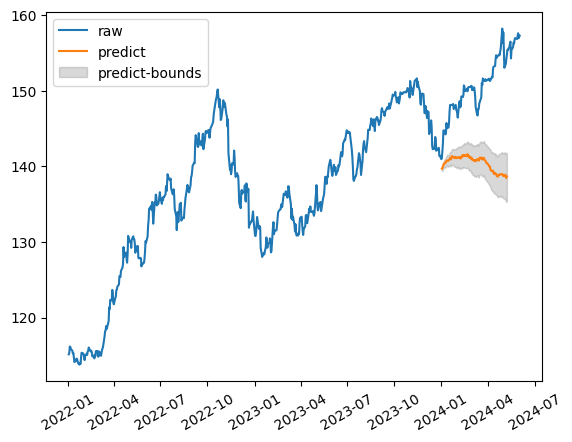
あまりうまく良くできているとは言えませんでした。
実験 為替USDJPY 日足 長期予測
次に長期の予測をやってみます。timesfmのhorizon_lenを512にして予測させてみます。
tfm = timesfm.TimesFm(
    context_len=1024,
    horizon_len=512,
    input_patch_len=32,
    output_patch_len=128,
    num_layers=20,
    model_dims=1280,
    backend="cpu",
)

tfm.load_from_checkpoint(repo_id="google/timesfm-1.0-200m")

import pandas as pd
df['ds'] = pd.to_datetime(df['ds'])
input_df = df.loc[('2015-01-01' <= df['ds']) & (df['ds'] <= '2023-01-01'), :]
forecast_df = tfm.forecast_on_df(
    inputs=input_df,
    freq="D",
    value_name="Close",
    num_jobs=-1,
)
import matplotlib.pyplot as plt

plot_df = df.loc[df['ds'] > '2022-01-01']
plt.plot(plot_df['ds'], plot_df['Close'], label='raw')
plt.plot(forecast_df['ds'], forecast_df['timesfm'], label='predict')
plt.fill_between(forecast_df['ds'], forecast_df["timesfm-q-0.4"], forecast_df["timesfm-q-0.6"], color='gray', alpha=0.3, label='predict-bounds')

plt.xticks(rotation=30)
plt.legend()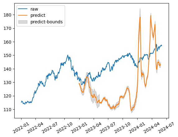
これもあまりいい予測ではありませんでした。予測が外れていることもそうですが、途中ピークを表す波形になってしまいました。
実験 為替USDJPY 1時間足 短期予測
1時間足を使った予測をしてみます。まず1時間足をyfinanceを使って取ってきます。yfinanceの仕様で、1時間足は最大で720daysまでしか取得できないので、periodを2yに設定します。
また、timesFMのforecast_on_df関数が、date型には対応していますが、datetime型には対応していなかったため、forecast関数で予測をします。
df = yf.download(tickers='USDJPY=X', interval='1h', period='2y')
df = df.reset_index().rename(columns={'Datetime':'ds'})
df['unique_id'] = 'USDJPY'
tfm = timesfm.TimesFm(
    context_len=512,
    horizon_len=128,
    input_patch_len=32,
    output_patch_len=128,
    num_layers=20,
    model_dims=1280,
    backend="cpu",
)

tfm.load_from_checkpoint(repo_id="google/timesfm-1.0-200m")
import pandas as pd
forecast_input = [
    df.loc[df['ds'] <= '2023-01-01', 'Close'].to_numpy()
]
frequency_input = [0]

point_forecast, experimental_quantile_forecast = tfm.forecast(
    forecast_input,
    freq=frequency_input,
)
import numpy as np
import matplotlib.pyplot as plt

x1 = np.arange(0, len(df))
plt.plot(x1, df['Close'], label='raw')

y2 = point_forecast[0, :]
x2 = np.arange(len(forecast_input[0]), len(forecast_input[0])+len(y2))
plt.plot(x2, y2, label='predict')
plt.legend(loc='lower left')

plt.xlim([len(forecast_input[0])-100, len(forecast_input[0])+len(y2)+100])

plt.xticks(rotation=30)
plt.legend()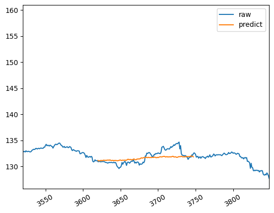
全く予測できていません。また、ほとんど予測値が変動していないため、当てにできません。
実験 為替USDJPY 1時間足 長期予測
長期間の予測はどうでしょうか?
df = yf.download(tickers='USDJPY=X', interval='1h', period='2y')
df = df.reset_index().rename(columns={'Datetime':'ds'})
df['unique_id'] = 'USDJPY'
tfm = timesfm.TimesFm(
    context_len=1024,
    horizon_len=512,
    input_patch_len=32,
    output_patch_len=128,
    num_layers=20,
    model_dims=1280,
    backend="cpu",
)

tfm.load_from_checkpoint(repo_id="google/timesfm-1.0-200m")
import pandas as pd
forecast_input = [
    df.loc[df['ds'] <= '2023-01-01', 'Close'].to_numpy()
]
frequency_input = [0]

point_forecast, experimental_quantile_forecast = tfm.forecast(
    forecast_input,
    freq=frequency_input,
)
import numpy as np
import matplotlib.pyplot as plt

x1 = np.arange(0, len(df))
plt.plot(x1, df['Close'], label='raw')

y2 = point_forecast[0, :]
x2 = np.arange(len(forecast_input[0]), len(forecast_input[0])+len(y2))
plt.plot(x2, y2, label='predict')
plt.legend(loc='lower left')

plt.xlim([len(forecast_input[0])-100, len(forecast_input[0])+len(y2)+100])

plt.xticks(rotation=30)
plt.legend()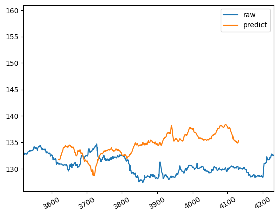
予測値は外れていますが、先程よりも変動しており、良くはなりました。
実験 為替USDJPY 1分足 長期予測
短期予測はあまりうまく行きそうにないので、長期予測だけ行いました。
df = yf.download(tickers='USDJPY=X', interval='1m')
df = df.reset_index().rename(columns={'Datetime':'ds'})
df['unique_id'] = 'USDJPY'
tfm = timesfm.TimesFm(
    context_len=1024,
    horizon_len=512,
    input_patch_len=32,
    output_patch_len=128,
    num_layers=20,
    model_dims=1280,
    backend="cpu",
)

tfm.load_from_checkpoint(repo_id="google/timesfm-1.0-200m")
import pandas as pd
forecast_input = [
    df.loc[df['ds'] <= '2024-05-30', 'Close'].to_numpy()
]
frequency_input = [0]

point_forecast, experimental_quantile_forecast = tfm.forecast(
    forecast_input,
    freq=frequency_input,
)
import numpy as np
import matplotlib.pyplot as plt

x1 = np.arange(0, len(df))
plt.plot(x1, df['Close'], label='raw')

y2 = point_forecast[0, :]
x2 = np.arange(len(forecast_input[0]), len(forecast_input[0])+len(y2))
plt.plot(x2, y2, label='predict')
plt.legend(loc='lower left')

plt.xlim([len(forecast_input[0])-100, len(forecast_input[0])+len(y2)+100])

plt.xticks(rotation=30)
plt.legend()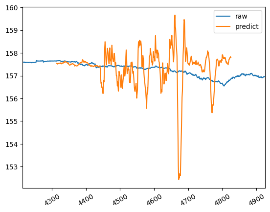
ぜんぜん駄目でした。振れ幅がひどすぎて、予測としては使えそうもありません。
まとめ
すべての実験で、予測はうまくいきませんでした。しかし、統計的に予測結果の良し悪しを算出していないので、もしかしたら、有効的に使える期間があるのかもしれません。
現状では、「明日の為替を知りたい」とか「数分後の為替を知りたい」とった用途では利用で来なさそうです。今後はパラメータなどの検証をやる気が湧いたらやります。