はじめに
TimesFMというのは200MパラメータをもつTransformerベースの時系列汎用予測モデルです。
大量の時系列データを学習することで、学習していないデータに対しても予測性能が高まったという研究内容ですね。
コードと動かし方は軽く書いてありますが、学術研究なので、ドキュメントなどは整備されていません。

今回はこれをDocker環境で使ってみたいと思います。
環境構築
Dev-containerを使っています。
構築ディレクトリはこんな感じ
.
├── .devcontainer
│   ├── Dockerfile
│   ├── devcontainer.json
│   ├── docker-compose.yml
│   └── requirements.txt
├── api_keys.json
└── notebooks
notebooksはjupyter-notebookのファイルを入れる場所です。
.devcontainer.json
拡張機能はpythonとjupyterだけです。必要に応じて追加してください。
{
    "name": "times_fm_project",
    "service": "stock_predict_by_timesfm",
    "dockerComposeFile": "docker-compose.yml",
    "remoteUser": "vscode",
    "workspaceFolder": "/work",
    "customizations": {
      "vscode": {
        "extensions": [
          "ms-python.python",
          "ms-toolsai.jupyter"
        ]
      }
    }
}
docker-compose.yml
composeで環境構築します。特に記載するべき注意点もないと思ます。
version: '3'
services:
  stock_predict_by_timesfm:
    container_name: 'stock_predict_by_timesfm_container'
    hostname: 'stock_predict_by_timesfm_container'
    build: .
    restart: always
    working_dir: '/work'
    tty: true
    volumes:
      - type: bind
        source: ..
        target: /work
Dockerfile
本家はanaconda環境でしたが、本記事ではpython3.10のslimを使います。
バージョンの依存関係がかなり厳格に決まっているので、3.10じゃないとだめだったと思います。
FROM python:3.10-slim-bullseye

ARG USERNAME=vscode
ARG USER_UID=1000
ARG USER_GID=$USER_UID

ENV LANG ja_JP.UTF-8
ENV LANGUAGE ja_JP:ja
ENV LC_ALL ja_JP.UTF-8
ENV TZ JST-9
ENV TERM xterm

RUN apt-get update \
    && groupadd --gid $USER_GID $USERNAME \
    && useradd -s /bin/bash --uid $USER_UID --gid $USER_GID -m $USERNAME \
    && apt-get install -y sudo \
    && echo $USERNAME ALL=\(root\) NOPASSWD:ALL > /etc/sudoers.d/$USERNAME \
    && chmod 0440 /etc/sudoers.d/$USERNAME \
    && apt-get -y install locales \
    && localedef -f UTF-8 -i ja_JP ja_JP.UTF-8

RUN apt-get -y install git

RUN pip install --upgrade pip
RUN pip install --upgrade setuptools

COPY ./requirements.txt .
RUN pip install -r requirements.txt
requirements.txt
バージョンの互換性が無いライブラリを使っていますし、timesfmのインストールの際もバーションの指定をしてくるので、かなり厳格に設定しました。
これを適当にやってエラー祭りになり、1日無駄にしました。
huggingface_hub[cli]==0.23.0
utilsforecast==0.1.9
utilsforecast ==0.1.9
praxis==1.4.0
lingvo==0.12.7
paxml==1.4.0
einshape==1.0
jax==0.4.26
jaxlib==0.4.26
numpy==1.26.4
pandas==2.2.2
git+https://github.com/google-research/timesfm.git

pandas_datareader
yfinance
xlrd
api_keys.json
apiキーを保存しておいてください。あとで直接書き込んでも構いません(今回はhuggingfaceのapiが一つなので、別で分ける理由は殆ど無いです)。
{
    "huggingface_hub":"xxx"
}
Sin波を予測してみる
まずはsin波を予測してみます。以下jupter-notebookのブロックと結果です。
はじめにtimesfmをロードしてみます。問題なく環境構築できていればエラーはでません。エラーがでた方は、環境構築とにらめっこしてください。
import timesfmただ、cuda環境ではないため、以下の警告がでましたが、問題なく使えます。
2024-05-18 14:32:29.843329: W tensorflow/stream_executor/platform/default/dso_loader.cc:64] Could not load dynamic library 'libcudart.so.11.0'; dlerror: libcudart.so.11.0: cannot open shared object file: No such file or directoryモデルを作ります。context_lenは入力長、horizon_lenは出力長です(おそらく)。2の累乗であることが望ましいと書かれていました。
tfm = timesfm.TimesFm(
    context_len=256,
    horizon_len=128,
    input_patch_len=32,
    output_patch_len=128,
    num_layers=20,
    model_dims=1280,
    backend="cpu",
)
huggingfaceのapiキーを入れて、huggingface_hubにログインします。
import json
with open('/work/api_keys.json', 'r') as f:
    api_keys = json.load(f)
from huggingface_hub import login
login(token = api_keys['huggingface_hub'])
成功すれば、Login successfulとでます。
モデルの学習済みの重みをロードします。上記のhuggingfaceのログインが成功していないと、ロードはできません。
tfm.load_from_checkpoint(repo_id="google/timesfm-1.0-200m")Sin波を作ります。合計三種類用意しました。上から、波長が短いもの、中くらいのもの、長いもののです。また、frequency_inputには、入力系列の波長タイプをintで指定します。
公式のには次のように書かれています。
- 0 (default): high frequency, long horizon time series. We recommend using this for time series up to daily granularity.
- 1: medium frequency time series. We recommend using this for weekly and monthly data.
- 2: low frequency, short horizon time series. We recommend using this for anything beyond monthly, e.g. quarterly or yearly.
また、株価や通貨などの実時間における波長タイプは次のように分類できるそうです(tickデータや分足、時間足、日足は0。週足や月足は1。年足は2)。
- 0: T, MIN, H, D, B, U
- 1: W, M
- 2: Q, Y
かなり、曖昧な区分のような気もしますが、どうなんでしょう?
import numpy as np
forecast_input = [
    np.sin(np.linspace(0, 20, 100)),
    np.sin(np.linspace(0, 20, 200)),
    np.sin(np.linspace(0, 20, 400)),
]
frequency_input = [0, 1, 2]
用意した入力データをモデルに入れます。
point_forecast, experimental_quantile_forecast = tfm.forecast(
    forecast_input,
    freq=frequency_input,
)
数十秒で予測値がでてきます。
予測値はpoint_forecastです。
実際の値と、予測値を見てみましょう。
import matplotlib.pyplot as plt
for n in range(len(forecast_input)):

    y1 = forecast_input[n]
    x1 = np.arange(len(y1))
    plt.plot(x1, y1, label='raw')

    y2 = point_forecast[n, :]
    x2 = np.arange(len(y1), len(y1)+len(y2))
    plt.plot(x2, y2, label='predict')
    plt.legend(loc='lower left')

    plt.show()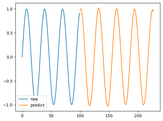
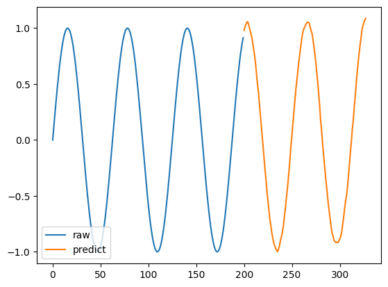

よく予測できていると言えるのではないでしょうか。
若干、折り返し地点が甘かったり、滑らかにならない場合があるのですが、学習せずに予測できる精度と考えると、良い気がします。
合成した関数ではどうでしょう。
sin波を適当に合成します。
x = np.linspace(0, 20, 400)
raw = [
    np.sin(2*x) + np.sin(4*x) + np.sin(8*x)
]
x = np.linspace(0, 10, 200)
forecast_input = [
    np.sin(2*x) + np.sin(4*x) + np.sin(8*x)
]
frequency_input = [0]
plt.plot(input[0])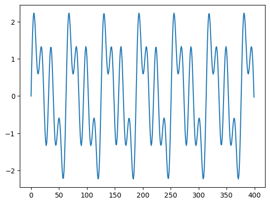
これの半分を入力してましょう。
point_forecast, experimental_quantile_forecast = tfm.forecast(
    forecast_input,
    freq=frequency_input,
)
y1 = raw[0]
x1 = np.arange(0, 400)
plt.plot(x1, y1, label='raw')
y2 = point_forecast[0, :]
x2 = np.arange(len(y1), len(y1)+len(y2))
plt.plot(x2, y2, label='predict')
plt.legend(loc='lower left')
plt.show()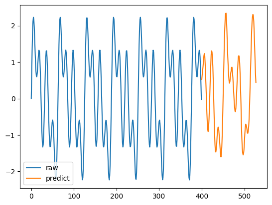
正しく予測できているとはいえませんね。しかし、ピーク値の予測はできているように感じます。
論文を読み込んでいないので、詳細な仕様がわからないのですが、入力する際に複数系列を入れたほうがよいのでしょうか?
先程の合成関数の他に、ばらした関数も入れてみましょう。
x = np.linspace(0, 20, 400)
raw = [
np.sin(2*x) + np.sin(4*x) + np.sin(8*x)
]
x = np.linspace(0, 10, 200)
forecast_input = [
np.sin(2*x) + np.sin(4*x) + np.sin(8*x),
np.sin(2*x),
np.sin(4*x),
np.sin(8*x)
]
frequency_input = [0, 0, 0, 0]
point_forecast, experimental_quantile_forecast = tfm.forecast(
forecast_input,
freq=frequency_input,
)
y1 = raw[0]
x1 = np.arange(0, 400)
plt.plot(x1, y1, label='raw')
y2 = point_forecast[0, :]
x2 = np.arange(len(y1), len(y1)+len(y2))
plt.plot(x2, y2, label='predict')
plt.legend(loc='lower left')
plt.show()
変わりませんね。複数系列を入れても、独立して予測しているようです。
追記
timesFMを使って株価予測した話を書きました。